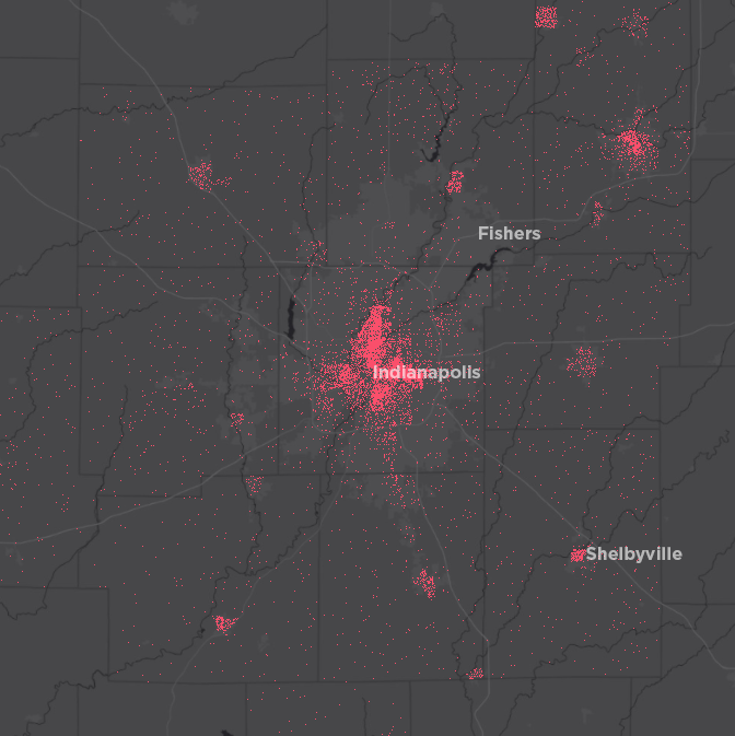
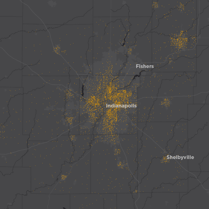
Housing Units Developed in Each Period
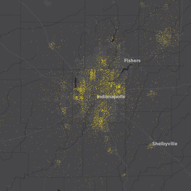
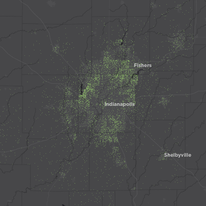
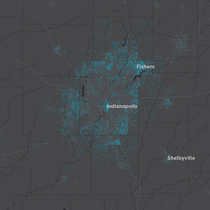
An Approach to Classifying Neighborhoods
The maps above provide a useful perspective, but how can we turn this into a neighborhood-level measure to classify areas by development period? Every tract has a mix of housing built in different time periods. However, if we classify areas based on the most common development period, a clear pattern starts to emerge.
For example, the tract that contains the State Fairgrounds had 322 units built before 1940, 550 built in the 1940s and 1950s, and 94 built in other periods. So we will classify this as predominantly built in the 1940s and 1950s.
This is a useful framework, but it presents some problems. The the center of Indianapolis and other cities and towns across the region were largely built before 1940 (red areas). But downtown Indianapolis is different, because some of its pre-war housing has been demolished. Newer housing built since 2000 now outnumbers the older housing stock. But it would be wrong to say that downtown Indy primarily developed in since 2000, since it is obviously the oldest part of the city.
A New Approach to Classifying Neighborhoods
If we also take into consideration the neighboring census tracts, we can start to develop more regular “bands” of development. Now, for example, by considering neighboring areas when we classify downtown Indy, we correctly find that the area is part of the old city core. This method has far fewer outliers and “stranded” tracts. The northeast side of Marion County, for example, is clearly split into three development bands instead of the mosaic of primary development periods shown in the previous attempt.
The downside of this approach is that outlying city centers are no longer classified as being primarily built before 1940, except in Anderson and Shelbyville. This is because units in newer developments outnumber the pre-war units in the core of many cities and towns across the region.
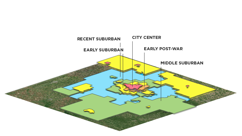
We call these resulting development bands City Center (primarily built before 1940), Early Post-War (1940s and 1950s), Early Suburbs (1960s and 1970s), Middle Suburbs (1980s and 1990s), and Recent Suburbs (2000s and 2010s).
Resulting Development Bands
Now that we have defined each development band, let’s analyze each.
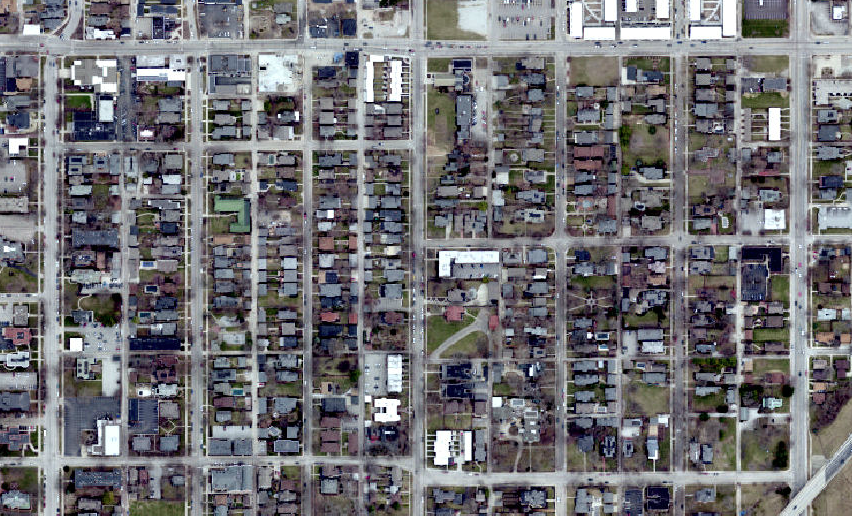
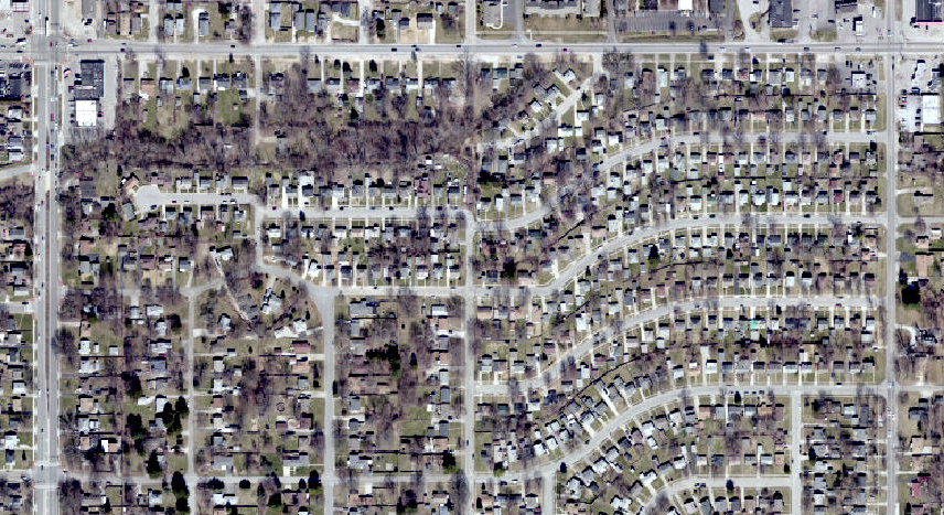
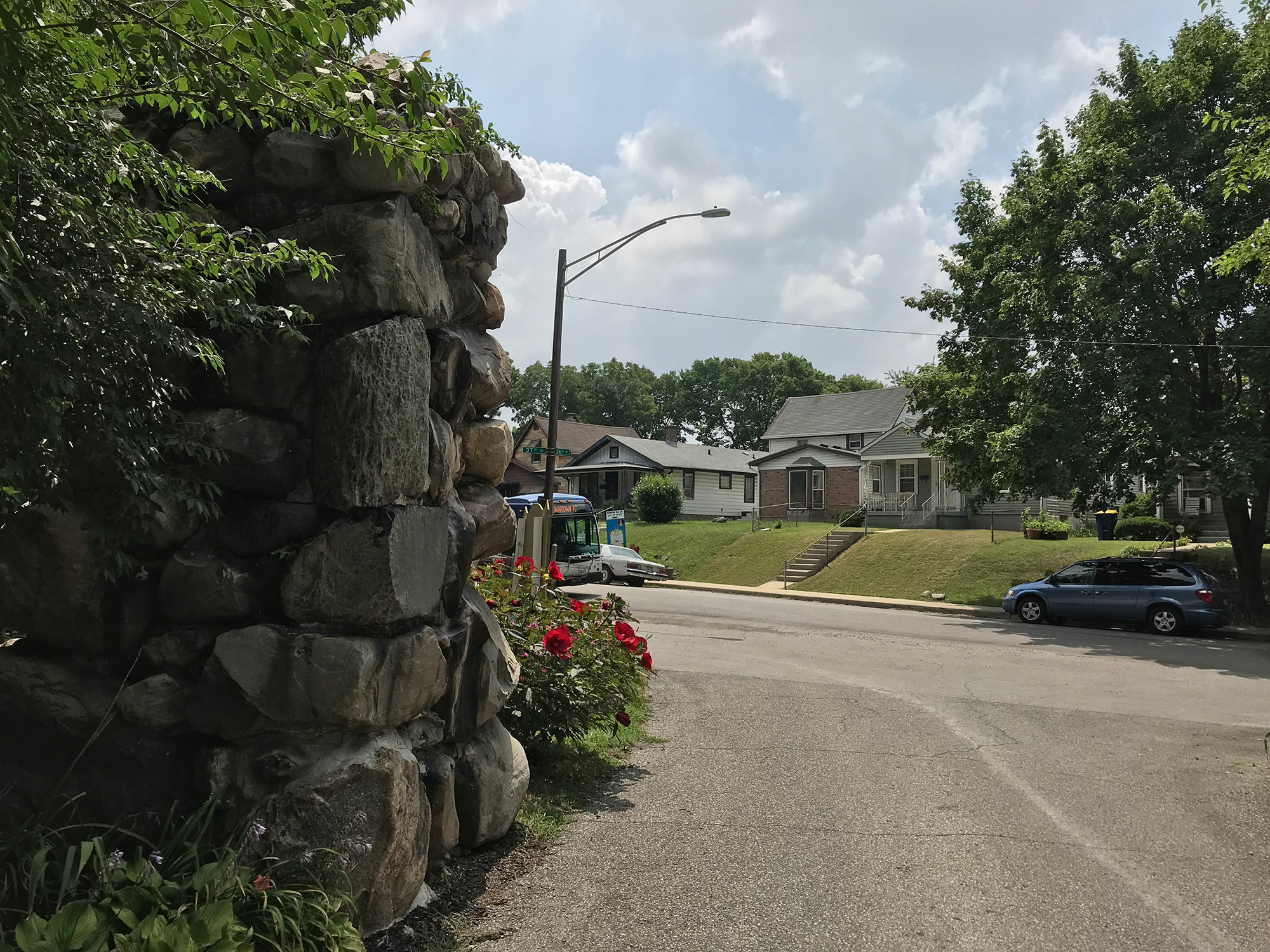
The City Center area makes up the core of Indianapolis, Anderson and Shelbyville. It accounts for 47 square miles, one percent of the regions area, but contains 93,639 housing units, 11 percent of the regions housing supply. The City Center band has a density of 2,005 housing units per square mile. Below is a typical neighborhood in the City Center area. Homes are typically brick or wood siding. If garages are present, they are along an alley. The street network is a grid system with high connectivity (many intersections).
Next Up
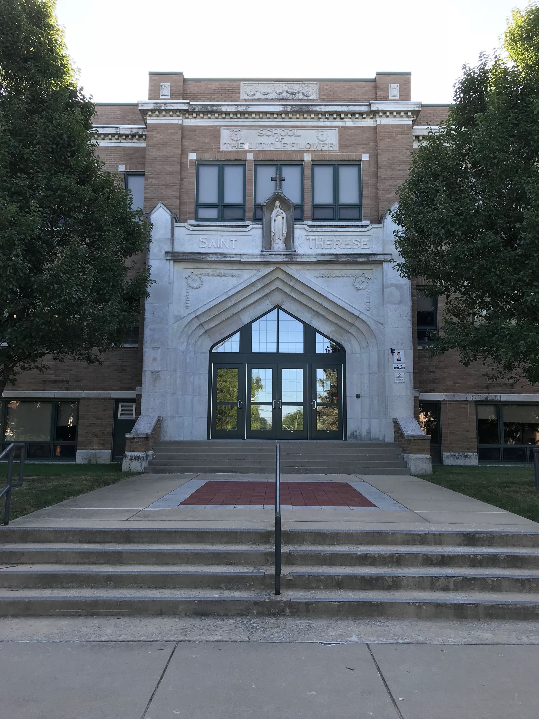 In Little Flower, More College Graduates, Young Adults, but Incomes are Falling
There’s a shrinking share of people in their 20s in this German/Irish neighborhood, but a growing of share in their 30s and 40s, as well as a growing population of children. These residents are less likely to live in poverty than other age groups, but they have still seen incomes decline 26 percent since 2010.
 Income Inequality High Where Golden Hill and Northwest Indianapolis Converge
In the area where wealthy Golden Hills converges with the working-class neighborhoods of Northwest Indianapolis, income inequality is high and increasing. The area is also experiencing a growth of white households above the median income.
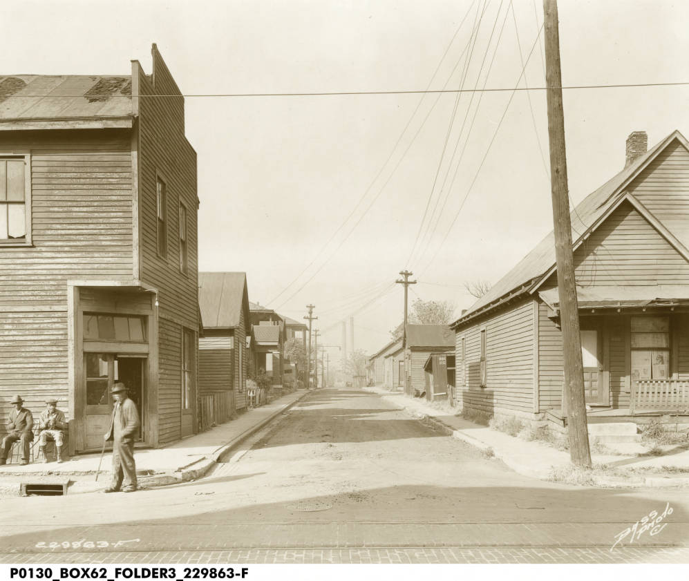 Changes in Indy’s Historic Black Neighborhoods
In the 1970s, 4,000 residents left this nearly all-black neighborhood. Why? An increasingly desegregated housing market and closure of one of the country’s first public housing projects.
 Story Map: Moving Out – Suburbanization Since 1970
Indianapolis and Anderson were the region’s urban centers in 1970. Three-quarters of the population lived in those counties. Now, just over half the population live there, and Hamilton County is the second largest urban center.